JAM Tutorial: 2D Laminar Flow Around a Cylinder
Contents
- Initial Setup
- Problem Configuration
- Derivative Definitions
- Compute symbolic functions
- Numerical Simulation: Domain Discretization
- Equation Pointers and Projection Matrices
- Variable Initialization
- Physical Grid Generation
- Full Variable Expansion
- Simulation Parameters and Initial Guess
- Time Integration Setup
- Main Simulation Loop (Newton-Raphson)
- Numerical resolution with the Newton-Raphson method
- Visualization
Initial Setup
Clears the workspace, restores default MATLAB paths, and sets up a subfolder 'equation/' for storing auxiliary functions. This ensures a clean environment and organizes generated function files.
clear all; % Clear workspace
restoredefaultpath; % Restore default MATLAB paths
pathequation = ['equation/'];%Symbolic equations
if ~isfolder(pathequation)
    mkdir(pathequation);
end
addpath([pwd '/' pathequation]); % Path for Jacobian functions
Problem Configuration
This section defines the physical parameters and computational domain for the 2D laminar flow around a cylinder problem.
A sketch of the physical problem is shown below:
The problem is formulated in dimensionless form using the incident velocity, cylinder radius, and fluid density. The primary independent physical parameter is the Reynolds number ( ). Other parameters define the computational domain geometry.
% List of physical and domain parameters
list_param = {'Re', 'Rout', 'L1', 'L2', 'Y1', 'X1', 'Y2', 'X2'};
Np = length(list_param);
The computational domain will be divided in two regions. In this particular example, in both region are each are defined the same unknowns, the velocity components in cartesian,  and
and  ; the pressure
  and
and  and
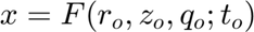
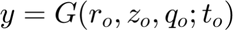
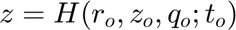
and  which relates the physical domain, (x,y,z), with the mapped one
 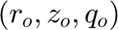 .
.
 is the corresponding time-variable in the mapped space. Note that in this present case
  does not appears because of the 2D character of the problem. We keep track also of the total number of the variables in the regions.
NRegion = 2; % Number of domain blocks (lower and upper)
list_var{1} = {'vy', 'vx', 'p', 'F', 'G'}; % Variables in block 1 (lower: y<0)
list_var{2} = {'vy', 'vx', 'p', 'F', 'G'}; % Variables in block 2 (upper: y>0)
list_varA = cat(2, list_var{:}); % All variables combined
NVAR = cellfun(@length, list_var); % Number of variables per block
NVA = length(list_varA); % Total number of variables

% In addition to the regions, 8 specific locations (boundaries/interfaces)
% are identified where the governing equations or boundary conditions
% may differ.
Nequations = 8; % Number of equation types in the domain
Derivative Definitions
Defines the types and orders of derivatives used in the equations. Derivatives are performed in the mapped computational space ( ). '' : No derivative. Single character (e.g., 'r0'): First-order derivative with respect to that variable (e.g.,
  ). The '0' indicates the mapped space. Repeated characters (e.g., 'rr0'): Higher-order derivative (e.g.,
  ). Multiple characters (e.g., 'rz0'): Mixed derivative (e.g.,
  ).
).
list_der0 = {'', 'r0', 'z0', 'rr0', 'zz0', 'rz0','t0'}; % Derivative types
NDA = length(list_der0); % Number of derivatives

% Generate symbolic representations for the derivatives (used internally
% by symbolic processing scripts).
list_dersymbolic{1} = '';
for i=2:NDA
    name=list_der0{i};
    out=[];
    for k=1:length(name)-1
        out = [out ',' name(k) '0'];
    end
    out = [out ')'];
    list_dersymbolic{i} = out;
end
Compute symbolic functions
This step derives the MATLAB functions for the problem's equations and their Jacobians using symbolic computation. This needs to be done only once unless the equations change. The flag `leq` controls whether this step is executed (1 to compile, 0 to skip). Symbolic parameters are created and then the blockA.m script performs the symbolic derivation.
leq=1; %compiling
if (leq==1)
    for i=1:Np
    pa(i,1)=sym(['pa_',num2str(i)],'real');
    eval(sprintf('%s = pa(%d);',list_param{i},i))
    end
    blockA;  %Symbolic calculation
    disp('Symbolic calcultations done!')
end
Numerical Simulation: Domain Discretization
Sets the number of nodes in the radial and axial directions for each region.
nr = [17, 17]; % Radial nodes per region
nz = [801, 801]; % Axial points per block (must be multiple of 4 + 1)
the numerical differentiation of a certain variable, v1, in the entire numerical domain is performed through the derivatives collocation matrices genenerated within collocationmatrices2th.m It also returns the indices (`Ia`, `Ib`, `Ja`, `Jb`) corresponding to the nodes within each region in the global discretized domain.
[r0A, z0A, nrA, nzA, ddr0A, ddrr0A, ddz0A, ddzz0A, Ia, Ib, Ja, Jb] = ...
    collocationmatrices2th(nr, nz, NRegion); % Generate collocation matrices

ntA = nrA * nzA; % Total grid points in full domain
nt = nr .* nz; % Grid points per block
Equation Pointers and Projection Matrices
The pointers.m script sets up indices and projection matrices required to map variables and equations between the regional and global domain representations and to apply boundary conditions.
pointers;
Variable Initialization
Initializes the solution variables ( ) for each region with zero values. These will be populated with an initial guess or previous solution.
idx = 1;
for k = 1:NRegion
    for v = 1:NVAR(k)
        eval(sprintf('%s%d = zeros(nr(%d), nz(%d));', list_varA{idx}, k, k, k));
        idx = idx + 1;
    end
end
Physical Grid Generation
Generates the physical coordinates (x, y) for the computational grid based on the defined domain parameters and mapping functions.
rA = repmat(r0A', 1, nzA); % Radial coordinates
zA = repmat(z0A, nrA, 1); % Axial coordinates
rrA{1} = repmat((r0A(1:nr(1))/r0A(1))', 1, nzA); % Normalized radial coords (block 1)
rrA{2} = repmat((r0A(nr(1):nrA)/r0A(nrA))', 1, nzA); % Normalized radial coords (block 2)

% Domain boundaries
Rout = 6; % Outer wall y-coordinate
L1 = 6; % Inlet x-coordinate
L2 = 16; % Outlet x-coordinate

% Mapping functions for grid
[~, j01] = min(abs(z0A - 0.25)); % Left stagnation point index
[~, j02] = min(abs(z0A - 0.5)); % Right stagnation point index
x1 = z0A(1:j01) / z0A(j01);
x2 = (z0A(j01:j02) - z0A(j01)) / (z0A(j02) - z0A(j01));
x3 = (z0A(j02:nzA) - z0A(j02)) / (z0A(nzA) - z0A(j02));
g0{1} = [-L1 + x1*(L1-1), -cos(pi*x2(2:end-1)), 1 + x3*(L2-1)]; % Block 1 x-mapping
f0{1} = [zeros(1, length(x1)), -sin(pi*x2(2:end-1)), zeros(1, length(x3))]; % Block 1 y-mapping
g1{1} = g0{1}; % Block 1 outer x-boundary
f1{1} = -Rout * ones(1, nzA); % Block 1 outer y-boundary
g0{2} = g0{1}; % Block 2 x-mapping
f0{2} = [zeros(1, length(x1)), sin(pi*x2(2:end-1)), zeros(1, length(x3))]; % Block 2 y-mapping
g1{2} = g0{1}; % Block 2 outer x-boundary
f1{2} = Rout * ones(1, nzA); % Block 2 outer y-boundary

% Generate initial mesh
for k = 1:NRegion
    z1 = zA(Ia(k):Ib(k), Ja(k):Jb(k));
    r1 = rrA{k};
    g00 = repmat(g0{k}, nr(k), 1);
    g11 = repmat(g1{k}, nr(k), 1);
    f00 = repmat(f0{k}, nr(k), 1);
    f11 = repmat(f1{k}, nr(k), 1);
    eval(sprintf('F%d = f00 + (f11 - f00) .* r1;', k)); % y-coordinates
    eval(sprintf('G%d = g00 + (g11 - g00) .* r1;', k)); % x-coordinates
end

% Combine borders for full domain
Y1 = [F1; zeros(nr(2)-1, nzA)]; % Block 1 y-border
X1 = [G1; zeros(nr(2)-1, nzA)]; % Block 1 x-border
Y2 = [zeros(nr(1)-1, nzA); F2]; % Block 2 y-border
X2 = [zeros(nr(1)-1, nzA); G2]; % Block 2 x-border
ndA = reshape(ndA, 1, ntA); % Flatten equation indices
Y1 = reshape(Y1, ntA, 1); % Flatten y-coordinates
Y2 = reshape(Y2, ntA, 1);
X1 = reshape(X1, ntA, 1); % Flatten x-coordinates
X2 = reshape(X2, ntA, 1);
Full Variable Expansion
Expands the initial/updated solution variables from their block-wise representation to the full global domain representation. This uses projection matrices (PNMv) generated in the `pointers.m` script.
lv = 0;
for k = 1:NRegion
    for i = 1:NVAR(k)
        lv = lv + 1;
        variable_name = list_var{k}{i};
        eval(sprintf('%s%dfull = reshape(PNMv{%d} * reshape(%s%d, ntv(%d), 1), nrA, nzA);', ...
            variable_name, k, lv, variable_name, k, lv));
    end
end
Simulation Parameters and Initial Guess
Sets the Reynolds number and the parameter vector. Calls a script (`redeabletoxooptima.m`) to prepare an initial guess for the solution vector (`x0` and `x0full`). Stores previous time step solutions for potential time integration schemes (although set up for a steady-state case here).
Re = 10; % Reynolds number
pa = [Re; Rout; L1; L2; 0; 0; 0; 0]; % Parameter vector
redeabletoxooptima; % Initial guess for x0 and x0full
x0mfull = x0full; % Previous time step solution
x0mmfull = x0mfull; % Previous-previous time step solution
Time Integration Setup
Sets up parameters for a generic second-order backward time integration scheme. However, for a steady-state problem, the time step (`dt`) is set to a very large value, effectively solving for the steady solution without actual time marching.

In case of equal timestep it reduces to,
In this case since we search a steady case (It is not a time evolution problem) we set  to infinity.
dt=1.e28;
dt1=dt;
ll is the time step and Ntimesteps is the number of timesteps. In the present case = 1 because stationary
Ntimesteps=1;

if(Ntimesteps>1)
tiempo(1) =0;
end
% The `tiempo` array would store the time instants for each step if Ntimesteps > 1.
Main Simulation Loop (Newton-Raphson)
This loop performs the simulation. For this steady-state case, it runs only once (Ntimesteps=1). Inside the loop, the nonlinear system of equations is solved using the Newton-Raphson iterative method.
for ll=1:Ntimesteps
    if (ll>1)
        tiempo(ll)=tiempo(ll-1)+dt;
    end
Numerical resolution with the Newton-Raphson method
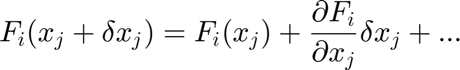
The Newton-Raphson method searchs to solve a nonlinear system of equations of the form, 
The Newton-Raphson results from a Taylor analysis around  ,
,
Demanding convergence,
The Newton-Raphson iterative method results,
or, in matrix form,
where  is the Jacobian tensor.
Initiallizing the error error and the number of iterations iter
    error=1e9;
    iter=0;
    nitermax = 150;
    errormax = 1e-3;
    relaxation = 0.5;
    while (error > errormax && iter < nitermax)
iter=iter+1;
Construct  and
and  with matrixAB.m
matrixAB;
Solve the linear system of equation to compute the correction  .
.
        dxa=a\b;
        error=max(abs(dxa))

        if(error > 10^8) error('Divergence detected'); end
Apply the correction
        x0=x0+relaxation*dxa;
        xotoredeableoptima; % Update variable
end
end
Visualization
velocity(G1, G2, F1, F2, vx1, vx2); % Plot x-velocity