Welcome to the JAM Tutorial

Contents

• Introduction to JAM
• Setting up the Environment
• Experimenting with the Examples
• Solving a problem with JAM step-by-step

Introduction to JAM

The Jacobian Analytical Method (JAM) is an advanced computational framework designed to efficiently solve complex non-linear problems, particularly those involving flows with free interfaces or moving boundaries. Originally developed by Herrada and Montanero (2016), JAM stands out for its ability to map intricate physical domains to rectangular spaces via non-singular transformations, simplifying both non-linear analysis and linear stability studies of capillary systems and other fluid dynamics problems.

What makes JAM unique is its focus on the symbolic computation of analytical Jacobians, eliminating the need for costly numerical approximations or the traditional use of Christoffel symbols to handle curvature in non-Euclidean spaces. This approach, refined in a recent work (Herrada, 2024), allows physical laws to be applied directly in Cartesian coordinates, even in curved domains, enhancing accuracy and reducing computational time.

Key features of JAM include:

• Analytical Jacobian Computation: Utilizes symbolic tools to derive Jacobians with high precision, minimizing numerical errors.
• Computational Optimization: Combines sparse collocation matrices with analytical Jacobians to assemble the numerical Jacobian matrix, speeding up Newton-Raphson iterations.
• Extreme Flexibility: Enables the construction of generalized eigenvalue problems to study the global stability of non-linear systems, adapting to diverse applications from capillary fluids to viscoelasticity.
• Avoids Christoffel Symbols: Simplifies formulation in curved spaces by projecting equations into Euclidean space, easing implementation and scalability.

JAM is particularly valuable in fields like fluid dynamics, where problems with free interfaces—such as liquid bridges, gravitational jets, or the breakup of viscoelastic threads—demand high precision and efficiency. Through this tutorial, you will learn how to implement JAM in Matlab or Python using practical examples available in the JAM GitHub repository. Get ready to discover a powerful tool that will transform your approach to numerical simulation!

Setting up the Environment

To run the JAM examples, you need to set up your environment with either Matlab or Python. Below are detailed instructions for installing and configuring both options, including the necessary dependencies.

Matlab Setup

Matlab requires a valid license to use. If you don’t have Matlab installed, follow these steps:

1. Download and install Matlab from the official MathWorks website: https://www.mathworks.com/products/matlab.html.
2. During installation, ensure you include the following toolboxes:
   • Symbolic Math Toolbox – Required for symbolic computation in JAM.
   • Optimization Toolbox – Essential for optimization tasks in JAM examples.
3. After installation, verify that these toolboxes are enabled. You can check this in Matlab by navigating to "Home" > "Add-Ons" > "Manage Add-Ons".

Python Setup

Python is a free, open-source alternative to Matlab. Below are instructions for installing Python, an IDE, and the required libraries on Windows 11 and Ubuntu.

Windows 11

1. Install Python:
   • Download the latest stable version of Python from https://www.python.org/downloads/.
   • Run the installer and ensure you check the box labeled "Add Python to PATH" to make Python accessible from the command line.
   • Complete the installation by following the on-screen instructions.
2. Install Visual Studio Code (IDE):
   • Download Visual Studio Code from https://code.visualstudio.com/.
   • Run the installer and follow the prompts to complete the installation.
   • Open Visual Studio Code, go to the Extensions view (Ctrl+Shift+X), search for "Python", and install the official Python extension by Microsoft.
3. Install Required Libraries:
   • Open a terminal in Visual Studio Code (Terminal > New Terminal) or use the Command Prompt.
   • Run the following command to install the necessary libraries:

     pip install numpy sympy scipy matplotlib

Ubuntu

1. Install Python:
   • Open a terminal and run the following commands to update your system and install Python along with pip:

     sudo apt update
     sudo apt install python3 python3-pip

2. Install Visual Studio Code (IDE):
   • Visual Studio Code is available on Ubuntu via the Snap package manager. Install it by running:

     sudo snap install --classic code

   • Open Visual Studio Code, go to the Extensions view (Ctrl+Shift+X), search for "Python", and install the official Python extension by Microsoft.
   • Alternative: If you prefer another IDE, you can install PyCharm Community Edition with:

     sudo snap install pycharm-community --classic

3. Install Required Libraries:
   • In the terminal, run the following command to install the necessary libraries:

     pip3 install numpy sympy scipy matplotlib

With Matlab or Python set up as described above, you’ll have all the tools and dependencies needed to run the JAM examples from the GitHub repository.

Experimenting with the Examples

To test the examples contained in the repository, you simply need to download them to your local directory. If you want to test an example in MATLAB, download the "Matlab" directory, open MATLAB, and navigate to the desired directory. For instance, you could go to the "elbow" directory. In JAM, the main program always starts with "Main". In this case, you would run the program Mainelbow3D.m. To run the same example in Python, download the "Python" directory to your computer and navigate to "elbow". Open your Python compiler (e.g., "Visual Studio Code") and execute the main file "Mainelbow3D.py". The symbolic functions required to assemble the numerical Jacobian are already generated and stored in the "Jacobians" directory of each example. The symbolic computation is performed by running the JAM function that always begins with "blockA". To see how these functions are generated, for MATLAB, you would run blockAcartesianvelocity.m , and for Python, "blockAelbow.py". The collocation matrices corresponding to the different types of discretizations that can be applied with JAM are located in the "utils/collocationmatrices" folder of the main directory.

Solving a problem with JAM step-by-step

2D Flow Around a Cylinder

As an example, we will solve the 2D flow of a liquid (incompressible fluid) with density \(\rho\) and viscosity \(\eta\) around a cylinder of radius \(R\), approaching from the left with a uniform velocity \(U\), and with the coordinate system \((x, y)\) originating at the center of the cylinder (see Figure 1). If we use \(U, \rho\), and \(R\) for nondimensionalization as characteristic magnitude the dimensionless equations for the bulk (regions [1] and [2] in the figure) are

• Continuity equation:

\[\nabla \cdot \mathbf{V} = 0\]

• Momentum equation:

\[\mathbf{M}_{\mathbf{X}} = \left( \frac{\partial \mathbf{V}}{\partial t} + (\mathbf{V} \cdot \nabla) \mathbf{V} \right) + \nabla p - \frac{1}{Re} \nabla^2 \mathbf{V} = \mathbf{0}\]

where, \(Re = \frac{\rho U R}{\mu}\) is the Reynolds number and all operators and vectors are written in the Cartesian system \(\mathbf{X}\).

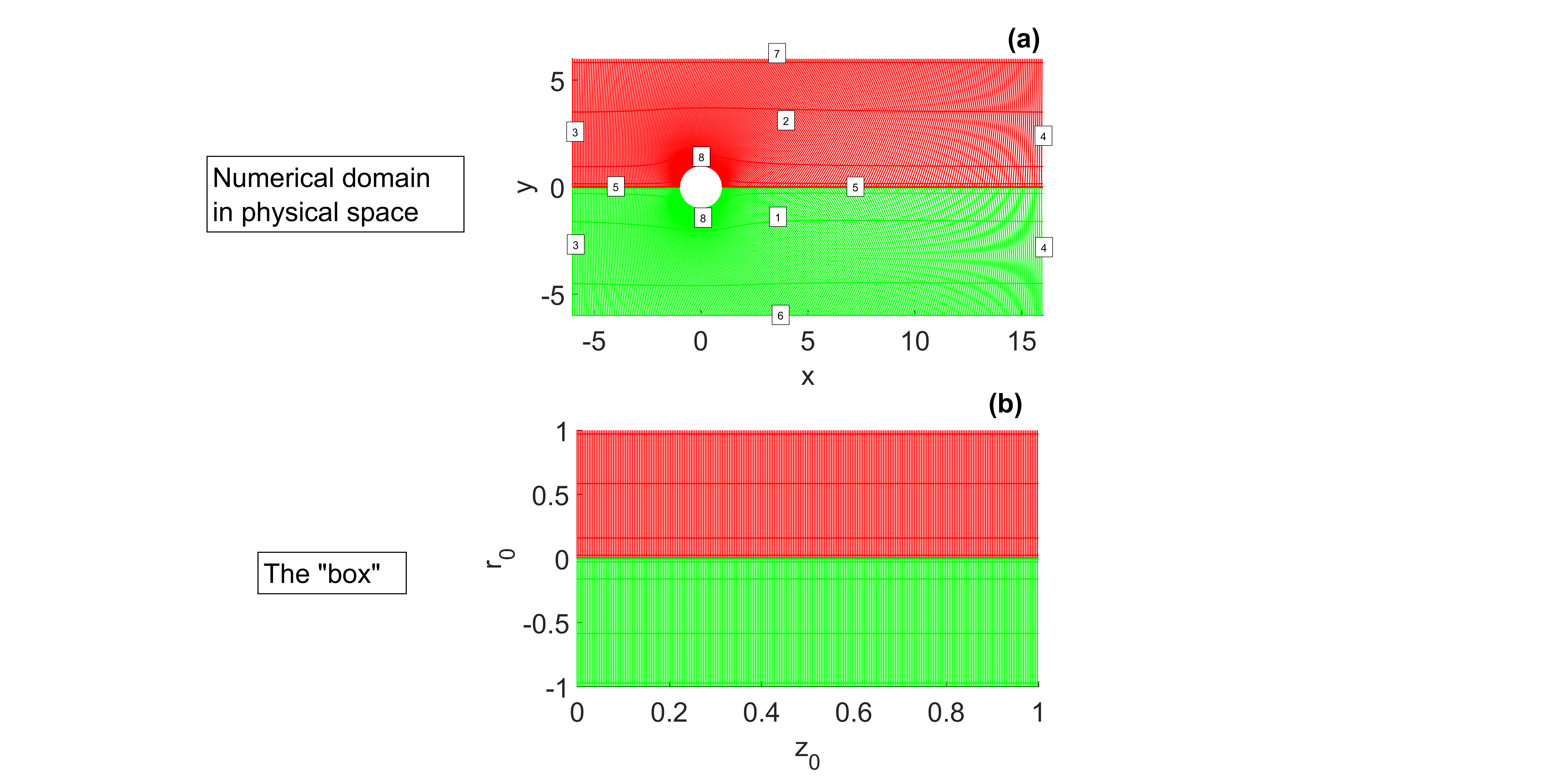
Our computational domain in the physical bidimensional space will be a rectangle \([-6 \times 16] \times [-6 \times 6]\) with the cylinder at the center. To map this domain to a rectangle \([0 \times 1] \times [-1 \times 1]\) in the transformed space \((z_0, r_0)\), we will apply two non-singular transformations between the upper/lower parts of the physical domain (red/green) and the upper/lower parts of our numerical "box" (see lines 157-171 in BlockA.m).

The \(z_0\) coordinate is discretized using \(nz\) finite differences of \(2^{(nd)}\) order (finites2thsparse.m function), while the \(r_0\) coordinates of the lower block and the upper block are discretized using Chebyshev polynomials with a stretching function controlled by parameter \(\alpha\) using chevitanh.m and chevitanh_inverse.m.

The resulting collocation matrices are discretizations in one dimension (\(z_0\) or \(r_0\)). One of the keys to applying the method is to extend these matrices to two or three dimensions. In our case, the 1D matrices are extended to 2D using the 'kron' command. The full 2D collocation matrices for each block are generated using the function collocationmatrices2th.m.

In order to obtain the eight variables in our discretized mesh, it is necessary to consider the lower block, for which four variables are required (\(vy_1, vx_1, p_1, F_1, G_1\)), and the upper block, for which four variables are required (\(vy_2, vx_2, p_2, F_2, G_2\)). In this case, \(vy\) denotes the velocity in the \(y\)-direction, \(vx\) the velocity in the \(x\)-direction, \(p\) denotes the \(y\)-position of the mesh points in the physical domain, and \(G\) denotes the \(x\)-position.

The variables contained within block 1(2) are defined exclusively within the green (red) dots in the box. The definition of both blocks of variables occurs solely at the connection points of the domains. The complete vector of unknowns, \(x_0\), resulting from the discretization of all unknowns, is initialized using the function redeabletoxooptima.m. This function also initializes the auxiliary function \(x_{ofull}\), which is an extension to all the points of the box (it takes as zero the variables that are not defined at the point).

As illustrated in Figure 1, eight different equations will be used depending on the position within the designated box: 1 and 2 (bulk), 3 (inlet), 4 (outlet), 5 (coupling between blocks 1 and 2), 6 (bottom wall), 7 (top wall), and 8 (cylinder wall). Within the function pointers.m, a pointer “ndA” is generated, which assigns the equation number to the spatial point and generates projection matrices between the box and subdomains 1 and 2 (PNM and PMN). The equations that are solved for each case are found in the BlockA.m function. These include the elliptic mappings for the bulk, mass and momentum conservation equations, and the boundary equations. The 'BlockA' function contains all the symbolic development necessary to generate the analytical functions we will need to assemble the Jacobian matrix in the matrixAB.m function.

The main code that allows us to obtain a stationary solution is Maincylinder.m, which is detailed below.

Results

After completing the simulation, the results can be visualized and analyzed to understand the behavior of the system. Below are some key aspects to consider when interpreting the results:

• Velocity Fields: Examine the velocity distribution in the domain to identify flow patterns, stagnation points, and regions of high shear.
• Pressure Distribution: Analyze the pressure contours to understand the forces acting on the fluid and the boundaries.
• Streamlines: Visualize the streamlines to observe the flow trajectories and identify recirculation zones.
• Validation: Compare the numerical results with analytical solutions or experimental data to validate the accuracy of the simulation.

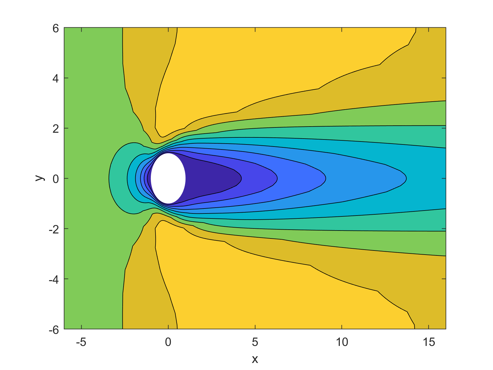
The visualization tools provided in the code, such as the velocity.m function, can be used to generate contours of the velocity components and other variables. For example, Figure 2 shows contours of the x-velocity for Re=10.

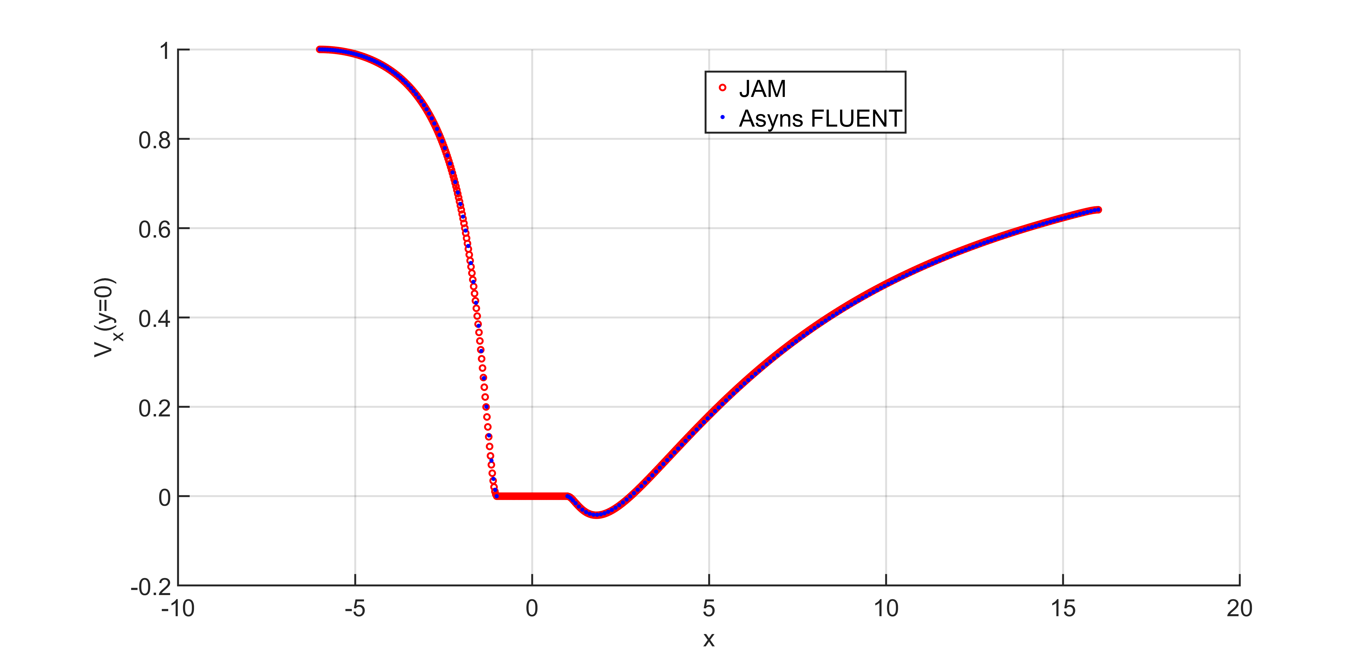
The solution obtained with JAM has been compared with the one obtained using the commercial code ANSYS FLUENT. Figure 3 shows the x-velocity along the axis (y=0) obtained with both codes.

By analyzing the results, you can gain insights into the physical phenomena being modeled and assess the performance of the JAM framework in solving complex problems.